Tutorial
This tutorial shows how to calculate RWB events step by step. After successfully installing WaveBreaking, the module needs to be imported. Make sure that the Python kernel with the correct virtual environment (where WaveBreaking is installed) is running.
import wavebreaking as wb
More information about the functions presented below can be found in the documentation.
Please note that the algorithm depends on the order of the spatial dimensions. Both the longitude and latitude dimensions should be in ascending order. Although the WaveBreaking tool identifies and adjusts descending coordinates, the dataset should be checked and adapted before starting the calculation to get the best performance.
Data pre-processing:
Optionally, the variable intended for the RWB calculations can be smoothed. The smoothing routine applies by default a 5-point smoothing (not diagonally) with a double-weighted center and an adjustable number of smoothing passes. Since the smoothing is based on the scipy.ndimage.convolve function, array-like weights and the mode for handling boundary values can be passed as an argument. This routine returns a xarray.DataArray with the variable “smooth_<variable>”.
# read data
import xarray as xr
demo_data = xr.open_dataset("tests/data/demo_data.nc")

# smooth variable with 5 passes
import numpy as np
smoothed = wb.calculate_smoothed_field(data=demo_data.PV,
                                       passes=5,
                                       weights=np.array([[0, 1, 0], [1, 2, 1], [0, 1, 0]]), # optional
                                       mode="wrap") # optional
The wavebreaking module calculates the intensity for each identified event, if an intensity field is provided. In my master thesis, the intensity is represented by the momentum flux derived from the product of the (daily) zonal deviations of both wind components. The routine creates a xarray.DataArray with the variable “mflux”. More information can be found in my master thesis.
# calculate momentum flux
mflux = wb.calculate_momentum_flux(u=demo_data.U,
                                   v=demo_data.V)
Contour calculation:
All RWB indices are based on a contour line representing the dynamical tropopause. The “calculate_contours()” function calculates the dynamical tropopause on the desired contour levels (commonly the 2 PVU level for Potential Vorticity). The function supports several contour levels at a time which allows for processing data of both hemispheres at the same time (e.g., contour levels -2 and 2). The contour calculation is also included in the RWB index functions and doesn’t need to be performed beforehand. However, you can also pass the contours directly to the index functions. This is especially useful if you want to perform the calculation of several indices at once.
If the input field is periodic, the parameter “periodic_add” can be used to extend the field in the longitudinal direction (default 120 degrees) to correctly extract the contour at the date border. With “original_coordinates = False”, array indices are returned (used for the index calculations) instead of original coordinates. The routine returns a geopandas.GeoDataFrame with a geometry column and some properties for each contour.
# calculate contours
contours = wb.calculate_contours(data=smoothed,
                                 contour_levels=[-2, 2],
                                 periodic_add=120, # optional
                                 original_coordinates=True) # optional
Index calculation:
All three RWB indices perform the contour calculation before identifying the RWB events. If you pass the separately calculated contours, the contour calcultion is skipped. For the streamer index, the default parameters are taken from `Wernli and Sprenger (2007)`_ (and `Sprenger et al. 2017`_) and for the overturning index from `Barnes and Hartmann (2012)`_. If the intensity is provided (momentum flux, see data pre-processing), it is calculated for each event. All index functions create a geopandas.GeoDataFrame with a geometry column and some properties for each event.
# calculate streamers
streamers = wb.calculate_streamers(data=smoothed,
                                   contour_levels=[-2, 2],
                                   contours=contours, #optional
                                   geo_dis=800, # optional
                                   cont_dis=1200, # optional
                                   intensity=mflux, # optional
                                   periodic_add=120) # optional
# calculate overturnings
overturnings = wb.calculate_overturnings(data=smoothed,
                                         contour_levels=[-2, 2],
                                         contours=contours, #optional
                                         range_group=5, # optional
                                         min_exp=5, # optional
                                         intensity=mflux, # optional
                                         periodic_add=120) # optional
# calculate cutoffs
cutoffs = wb.calculate_cutoffs(data=smoothed,
                               contour_levels=[-2, 2],
                               contours=contours, #optional
                               min_exp=5, # optional
                               intensity=mflux, # optional
                               periodic_add=120) # optional
Event classification:
The event classification is based on selecting the events of interest from the geopandas.GeoDataFrame provided by the index calculation functions.
Some suggested classifications:
# stratospheric and tropospheric (only for streamers and cutoffs)
stratospheric = events[events.mean_var >= contour_level]
tropospheric = events[events.mean_var < contour_level]

# anticyclonic and cyclonic by intensity for the Northern Hemisphere
anticyclonic = events[events.intensity >= 0]
cyclonic = events[events.intensity < 0]

# anticyclonic and cyclonic by intensity for the Southern Hemisphere
anticyclonic = events[events.intensity <= 0]
cyclonic = events[events.intensity > 0]

# anticyclonic and cyclonic by orientation (only for overturning events)
anticyclonic = events[events.orientation == "anticyclonic"]
cyclonic = events[events.orientation == "cyclonic"]
In addition, a subset of events with certain characteristics can be selected, e.g. the 10% largest events:
# 10 percent largest events
large = events[events.event_area >= events.event_area.quantile(0.9)]
Transform to DataArray:
To calculate and visualize the occurrence of RWB events, it comes in handy to transform the coordinates of the events into a xarray.DataArray. The “to_xarray” function flags every grid cell where an event is present with the value 1. Before the transformation, it is suggested to classify the events first and only use for example stratospheric events.
# classify events
stratospheric = streamers[streamers.mean_var.abs() >= 2]

# transform to xarray.DataArray
flag_array = wb.to_xarray(data=smoothed,
                          events=stratospheric)
Visualization:
WaveBreaking provides two options to do a first visual analysis of the output. Both options are based on the xarray.DataArray with the flagged grid cells from the “to_xarray” function.
To analyze a specific large scale situation, the RWB events on a single time steps can be plotted:
# import cartopy for projection
import cartopy.crs as ccrs

wb.plot_step(flag_data=flag_array,
             step="1959-06-05T06", #index or date
             data=smoothed, # optional
             contour_level=[-2, 2], # optional
             proj=ccrs.PlateCarree(), # optional
             size=(12,8), # optional
             periodic=True, # optional
             labels=True,# optional
             levels=None, # optional
             cmap="Blues", # optional
             color_events="gold", # optional
             title="") # optional

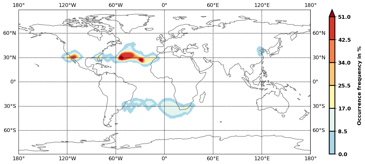
The analyze Rossby wave breaking from a climatological perspective, the occurrence (for specific seasons) can be plotted:
wb.plot_clim(flag_data=flag_array,
             seasons=None, # optional
             proj=ccrs.PlateCarree(), # optional
             size=(12,8), # optional
             smooth_passes=0, # optional
             periodic=True, # optional
             labels=True, # optional
             levels=None, # optional
             cmap=None, # optional
             title="") # optional
Event tracking:
Last but not least, WaveBreaking provides a routine to track events over time. Beside the time range of the temporal tracking, two methods for defining the spatial coherence are available. Events receive the same label if they either spatially overlap (method “by_overlapping”) or if the centre of mass lies in a certain radius (method “by_radius”). Again, it is suggested to classify the events first and only use for example stratospheric events. This routine adds a column “label” to the events geopandas.GeoDataFrame.
# classify events
anticyclonic = overturnings[overturnings.orientation == "anticyclonic"]

# track events
tracked = wb.track_events(events=anticyclonic,
                            time_range=6, #time range for temporal tracking in hours
                            method="by_overlap", #method for tracking ["by_overlap", "by_distance"], optional
                            buffer=0, # buffer in degrees for polygons overlapping, optional
                            overlap=0, # minimum overlap percentage, optinal
                            distance=1000) # distance in km for method "by_distance"
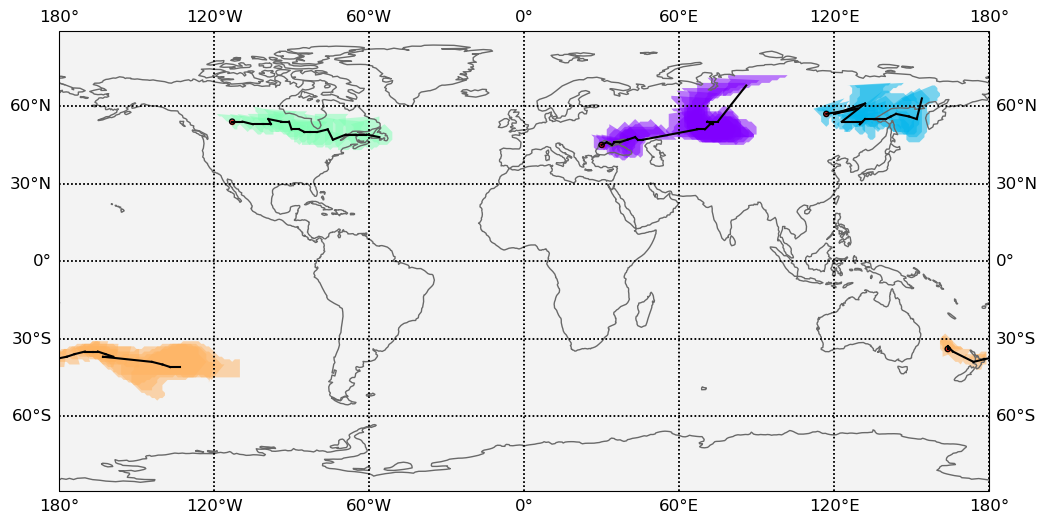
The result can be visualized by plotting the paths of the tracked events:
wb.plot_tracks(data=smoothed,
               events=tracked,
               proj=ccrs.PlateCarree(), # optional
               size=(12,8), # optional
               min_path=0, # optional
               plot_events=True, # optional
               labels=True, # optional
               title="") # optional